Agricultural Productivity in the United States - Methods

Note: Find the full citations for papers listed below in References. Find tables referenced below in the main file listing page.

USDA's Economic Research Service (ERS) has constructed accounts for the farm sector that are consistent with a gross output model of production (see Shumway et al. 2017, Ball et al. 2016). Output is defined as gross production leaving the farm, as opposed to real value added. Inputs are not limited to labor and capital but include intermediate inputs. Intermediate goods that are produced and consumed within the farm are self-cancelling transactions and, therefore, do not enter either output or input accounts.

ERS defined the farm sector in the same way as in the National Income and Product Accounts (NIPA). This definition means that minor goods and services (i.e., secondary outputs) for agriculture that are primary good and services for other industries were included in the primary industry’s output.

There are a few exceptions in the national productivity statistics, however, for which we take the existence of certain (inseparable) secondary activities into account when measuring the productive activity of the sector. These activities are defined as activities whose costs cannot be separately observed from those of the primary agricultural activity (see United Nations Revised System of National Accounts, 2008). Examples include machine services for hire, custom feeding of livestock, farm forestry, and recreational activities involving the means of production. The output of the sector thus results from two kinds of activities: agricultural activities, (whether primary or secondary), and non-agricultural activities of farms.

The next section is organized by component measures. Except where indicated, the methods described apply equally to States and the U.S. farm sector:

Output
Intermediate Input
Labor Input
Capital Input
Total Factor Productivity
Strengths and Limitations
Suggested Citation

Output

The output measure begins with disaggregated data for physical quantities and market prices of agricultural goods. The output quantity for each crop and livestock category consists of quantities of commodities sold off the farm (including unredeemed Commodity Credit Corporation loans), additions to inventory, and quantities consumed as part of final demand in farm households during the calendar year. Off-farm sales in the aggregate accounts are defined only in terms of output leaving the sector, while off-farm sales in the State accounts also include sales to the farm sector in other States.

The corresponding price reflects the value of that output to the producer, as subsidies are added and indirect taxes are subtracted from market values. The measure of output also includes goods and services of non-agricultural (or secondary) activities when these activities cannot be distinguished from the primary agricultural activity. Törnqvist indices of output are formed by aggregating over agricultural goods output and the output of goods and services of inseparable secondary activities using revenue-share weights on shadow prices—the prices farmers actually receive or face for each commodity that reflects the market value, the Government subsidy, and/or Government tax (or tax rebate) for that commodity as indicated above.

Intermediate Input

Intermediate input consists of goods used in production during the calendar year, whether withdrawn from beginning inventories or purchased from outside the farm sector or, in the case of the State production accounts, from farms in other States. Open-market purchases of feed and seed inputs enter both State and aggregate farm sector intermediate inputs accounts. Withdrawals from producers' inventories are also measured in output, intermediate input, and capital input. Beginning inventories of crops and livestock represent capital inputs and are treated in the discussion of capital below. Additions to these inventories represent deliveries to final demand and are treated as part of output. Goods withdrawn from inventory are symmetrically defined as intermediate inputs and recorded in the farm input accounts.

Data are compiled for each State current dollar consumption of petroleum fuels, natural gas, and electricity in agriculture for the period 1960–2004, and for 1948–2023 at the national level. Prices of individual fuels are taken from the Energy Information Administration's Monthly Energy Review. The index of energy consumption is formed implicitly as the ratio of total expenditures (less State and Federal excise tax refunds) to the corresponding price index.

Pesticides and fertilizers have undergone significant changes in quality over the study period (Fernandez-Cornejo et al., 2014). To measure input price and quantity in constant-efficiency units, we construct price indices for fertilizers and pesticides using hedonic methods. Under this approach, a good or service is viewed as a bundle of characteristics which contribute to the productivity (utility) derived from its use. Its price represents the valuation of the characteristics "that are bundled in it," and each characteristic is valued by its "implicit" price (Rosen, 1974). However, these prices are not observed directly and must be estimated from the hedonic price function.

A hedonic price function expresses the price of a good or service as a function of the quantities of the characteristics it embodies. Thus, the hedonic price function for pesticides, for example, may be expressed as W_p = W(X, D), where W_p represents the price of pesticides, X is a vector of characteristics or quality variables, and D is a vector of other variables that may affect price.

Kellogg et al. (2002) have compiled data on characteristics that capture differences in pesticide quality. These characteristics include toxicity, persistence in the environment, and leaching potential, among others.

Other variables (denoted by D) are also included in the hedonic equation, and their selection depends not only on the underlying theory but also on the objectives of the study. If the main objective of the study is to obtain price indices adjusted for quality, as in our case, the only variables that should be included in D are time or State dummy variables, which will capture all price effects other than quality. After allowing for differences in the levels of the characteristics, the part of the price difference not accounted for by the included characteristics will be reflected in the coefficients on the dummy variables.

Economic theory places few if any restrictions on the functional form of the hedonic price function. We adopt a generalized linear form, where the dependent variable and each of the continuous independent variables are represented by the Box-Cox transformation. This is a mathematical expression that assumes a different functional form depending on the transformation parameter, and which can assume both linear and logarithmic forms, as well as intermediate non-linear functional forms.

Thus, the general functional form of our hedonic model is given by:

$Equation: W_p(\lambda_0)=\sum_{n}^{ }\alpha_nX_n(\lambda _n)+\sum_{d}^{ }\gamma _dD_d+\varepsilon,$

where

$Equation: W_p(\lambda_0)$

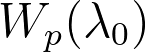
is the Box-Cox transformation of the dependent price variable, Wp > 0; that is,

Similarly,

is the Box-Cox transformation of the continuous quality variable X_n, where

and

Variables represented by D are time dummy variables, not subject to transformation;

and

are unknown parameter vectors, and

is a random error term.

Finally, price and implicit quantity indices are constructed for purchased services (such as purchased contract labor services, purchased machine services, and maintenance and repairs). Available data are limited to nominal expenditures for various services. To decompose expenditures for contract labor services into price and quantity components, we estimate a hedonic wage function where hourly earnings are expressed as a function of demographic characteristics (including sex, age, education, and experience), as well as legal status using National Agricultural Worker Survey data (see Wang et al., 2013b for further discussion). Purchased machine services substitute for own capital input. Therefore, we construct the implicit quantity of purchased machine services as the ratio of expenditures to an index of rental prices of agricultural machinery (i.e., farm tractors or agricultural machinery excluding tractors). Translog indices of intermediate input are constructed by weighting the growth rates of each category of intermediate input described above by their value share in the overall value of intermediate inputs.

Labor Input

There are three principal farm-labor related categories: self-employed and unpaid family labor, hired labor, and labor obtained through contract services. In the ERS productivity accounts, the labor input category includes the first two, while contract labor service is included in intermediate inputs, as a part of purchased services as indicated in the intermediate inputs section.

USDA farm labor accounts cross classify the agricultural workforce by demographic characteristics such as age, sex, education, experience, and employment type. These characteristics show how these attributes relate to one another and incorporate detailed demographic information into labor measurements. Using this framework, USDA has developed matrices of hours worked and hourly compensation for workers categorized by sex, age, education, and employment class (which distinguishes between employees, the self employed, and unpaid family labor).

This process was accomplished by incorporating data from both establishment and household surveys using the Response Analysis Survey (RAS) procedure (see Jorgenson et al., (1987:72–76) for more discussion). The farm sector matrices with demographic information were taken from the Census of Population (U.S. Department of Commerce, U.S. Bureau of the Census) and the American Community Survey (ACS). The resulting estimates of employment, hours worked, and labor compensation are regressed against the total numbers for the farm sector based on establishment surveys that underlie the U.S. National Income and Product Accounts (NIPA) and special tabulation work by the Bureau of Labor Statistics (BLS) derived from the Current Population Survey (CPS).

In addition, ERS has developed a set of similarly formatted but otherwise demographically distinct matrices of labor input and labor compensation by State. This process was accomplished using the RAS procedure (Jorgenson et al., (1987)) by combining the aggregate farm sector matrices with State-specific demographic information that is available from the decennial Census of Population (U.S. Department of Commerce) and the American Community Survey (for years after 2005). In the past, total hours worked at the State level used in the State productivity accounts were drawn from the USDA, NASS Farm Labor Survey (FLS). However, the questions on self-employed and unpaid family workers were discontinued in 2003, hindering their development in the State productivity accounts. While the Current Population Survey (CPS) is a replacement for self-employed and unpaid worker data source in the national accounts, the CPS State sample size is insufficient to provide reliable hours worked by self-employed and unpaid workers in the farm sector. After exploring various survey data sources (see Wang et al. 2025 for more details) and conducting statistical tests for comparison and robustness, the Agricultural Resource Management Survey (ARMS) was selected as the most suitable replacement source for the State-level self-employed and unpaid workers data. This decision was based on the statistical consistency of the hours worked distribution among States and the total hours estimates for self-employed and unpaid workers, which align more closely with the FLS than other sources.

However, because the survey design and weighting scheme differ between the FLS and ARMS, there is a discrepancy between the State estimates from the two surveys. Therefore, we used 2002 as the benchmark to develop the data on State hours worked to be consistent with the historical data. The result is a complete State-by-year panel data set of annual hours worked and hourly compensation matrices, with cells cross-classified by education and employment class (sex and age are not included in the demographic matrices for statistical reliable cross-classified estimates) and with each matrix regressed against the USDA hours-worked and compensation totals, respectively.

Indices of labor input were constructed for each State and the aggregate farm sector using the demographically cross-classified hours and compensation data (see Wang et al., 2024, 2025 for details). Labor hours having higher marginal productivity (e.g., wages) are given higher weights in forming the index of labor input than are hours having lower marginal productivities. Doing so explicitly adjusts indices of labor input for "quality" change in labor hours, as originally defined by Jorgenson & Griliches (1967).

Capital Input

Capital assets are long-lived assets that contribute to production over several years. In the productivity accounts, capital input is a measure of the service flow provided by an array of different capital assets, (including farm buildings and structures, machinery, breeding stock and other inventories, and land).

Construction of capital input and capital service prices for each State and the aggregate farm sector begins with estimating the capital stock and rental price for each asset type. For depreciable assets, the perpetual inventory method (United Nations, 2008) is used to develop stocks from data on investment. For land and inventories, capital stocks are measured as implicit quantities derived from balance sheet data from the Farm Income aggregate account. Implicit rental prices for each asset are based on the correspondence between the purchase price of the asset and the discounted value of future service flows derived from that asset.

Depreciable Assets

Under the perpetual inventory method, capital stock at the end of each period, K_t , is measured as the sum of all past investments, each weighted by its relative efficiency, d_τ:

where

$Equation: {d}_{\tau}$

is approximated by a hyperbolic efficiency function

and where L is the service life of the asset, τ represents the asset's age, and β is a curvature or decay parameter. We assume average service lives of 10 years for automobiles, 9 years for farm tractors, 17 years for other machinery, and 38 years for buildings. The value of β is restricted to values that are less than or equal to one. For values of β greater than zero, the efficiency of the asset approaches zero at an increasing rate. For values less than zero, efficiency approaches zero at a decreasing rate.

Little empirical evidence is available to suggest a precise value for β. However, two studies (Penson et al., 1977 and Romain et al., 1987) provide evidence that efficiency decay occurs more rapidly in the later years of service, corresponding to a value of β in the 0 to 1 interval. We assumed that the efficiency of a structure declines slowly over most of its service life until a point is reached where the cost of repairs exceeds the increased service flows derived from the repairs, at which point the structure is allowed to depreciate rapidly (β=0.75). The decay parameter for durable equipment (β=0.5) assumes that the decline in efficiency is more uniformly distributed over the asset's service life.

Consider now the efficiency function that holds β constant and allows L to vary. This concept of variable service lives is related to the concept of investment, where investment is a bundle of different types of capital goods. Each of the different types of capital goods is a homogeneous group of assets in which the actual service life, L , is a random variable reflecting quality differences, maintenance schedules, etc. For each asset type, there exists some mean service life, L ̅, around which there exists some distribution of actual service lives. To determine the amount of capital that is available for production, the actual service lives and their frequency of occurrence must be determined. It is assumed that the underlying distribution is the normal distribution truncated at points two standard deviations above and below the mean service life. Mean service lives correspond to 85 percent of the U.S. Department of the Treasury’s "Bulletin F" lives (U.S. Department of Treasury, 1961).

Capital Rental Prices

Firms will add to their capital stock so long as the present value of the net revenue generated by an additional unit of capital exceeds the purchase price of the asset. This formula can be stated algebraically as:

where p is the price of output (y),

is the marginal product of capital K so the gross revenue in each period will rise by

with an additional unit of K. Note that w_K is the price of investment assets and

is the increase in replacement (R) in period t required to maintain the capital stock at the new level. Thus net revenue will rise by:

Note that r is the real discount rate. To maximize net present value, firms will continue to add to capital stock until this equation holds as an equality (Ball et al., 2016):

where c is defined as the implicit rental price of capital.

The rental price consists of two components. The first term, rw_K, represents the opportunity cost associated with the initial investment. The second term,

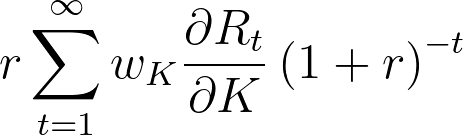
$Equation: {r}\sum_{t=1}^{\infty}{w}_{K}\frac{\partial{R}_{t}}{\partial{K}}\left(1+r\right)^{-t}$

-- is the present value of the cost of all future replacements that are required to maintain the productive capacity of the capital stock.

Let F denote the present value of the stream of capacity depreciation on one unit of capital according to the mortality distribution m:

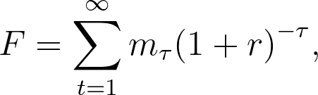
$Equation: F=\sum_{t=1}^{\infty}{m}_{\tau}{\left(1+r \right)}^{-\tau},$

where r = 1, ..., t

Since replacement at time t is equal to capacity depreciation at time t:

$Equation: \sum_{t=1}^{\infty}\frac{\partial{R}_{t}}{\partial{K}}\left(1+r\right)^{-t}=\sum_{t=1}^{\infty} {F}^{t}=\frac{F}{(1-F)}$

so that

$Equation: c=\frac{r{w}_{K}}{(1-F)}.$

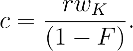
The real rate of return, r in the above expression, is calculated as the nominal yield on investment grade corporate bonds less the rate of inflation as measured by the asset specific prices. An ex-ante rate is then obtained by expressing observed real rates as an autoregressive integrated moving average (ARIMA) process. We calculate F holding the required real rate of return constant for that vintage of capital goods. In this way, implicit rental prices c are calculated for each asset type (except for inventory, for consistency, where the rate of inflation is measured by the implicit price deflator for gross domestic product). Asset prices and investment data are drawn from BLS, ERS, and NASS.

Finally, indices of capital input for each State and the aggregate farm sector are constructed by aggregating over the different capital assets, using the asset-specific rental prices as weights.

Land Input

Agricultural land (farmland) consists primarily of land used for crops, pasture, or grazing but also includes acres of idled cropland and woodland. In the ERS productivity accounts, land stock is measured as the real value of total farmland, which is nominal land value that is deflated by a land price index at the national level for aggregate land accounts and the State level for State land accounts.

To obtain a constant-quality stock of land, we compile data on land area and average value (excluding buildings) per acre for each county in each State. The land area in each county is drawn from the Census of Agriculture. Data for years intermediate to the censuses are estimated using cubic spline interpolation. However, the Census only reports data on the value of farm real estate (i.e., land and structures); it does not provide data on land values separately. Historically, the value of farm real estate was partitioned into its components using information from the Agricultural Economics and Land Ownership Survey (AELOS). However, AELOS was last conducted in 1999. We now rely on the annual USDA, Agricultural Resource Management Survey to derive estimates of the value of land from data on the value of farm real estate.

Differences in the quality of land across States and regions prevent the direct comparison of observed prices. To account for these quality differences, we calculate relative prices of land from hedonic regression results.

Consistent with the description above, the hedonic approach views land as a bundle of characteristics which contribute to output derived from its use. The World Soil Resources Office of the USDA's Natural Resources Conservation Service (NRCS) has compiled data on land characteristics (see Eswaren et al., (2003)). They develop a procedure for evaluating inherent land quality, and use this procedure to assess land resources on a global scale. Given the Eswaren et al., database, we use GIS to overlay State and county boundaries. The result of the overlay gives us the proportion of land area of each county in so-called soil stress categories. These characteristics include soil acidity, salinity, and moisture stress, among others. The "level" of each characteristic is measured as the percentage of the land area in a given region that is subject to stress. A detailed description of the characteristics included in this hedonic model is provided in Ball et al. (2008). The environmental attributes that are most highly correlated with land prices in major agricultural areas are moisture stress and soil acidity. In areas with extreme and persistent moisture stress, agriculture is generally not possible without irrigation. Hence irrigation (i.e., the percentage of the cropland that is irrigated) is included as a separate variable. Because irrigation mitigates the negative impact of soil acidity on plant growth, the interaction between irrigation and soil acidity is included in the vector of characteristics (Ball et al., 2008).

Total Factor Productivity

National-level Total Factor Productivity

The USDA model of total factor productivity (TFP) growth is based on a translog transformation frontier. The model relates the revenue-share-weighted growth rates of multiple outputs to the cost-share-weighted growth rates of labor, capital, and intermediate inputs. TFP growth is the difference between the growth of aggregate output and the growth of all inputs taken together. We measured TFP growth using the Törnqvist index number approach. TFP growth over two time periods was defined as:

where R_it are output revenue shares, Y_it are individual outputs, W_jt are input cost shares, X_jt are individual inputs, t and t-1 and denote the current and previous year, i denotes the ith output, and j denotes the jth input (see Wang et al. 2024a for details).

State-level Total Factor Productivity

We first constructed normalized multilateral prices and quantities for outputs (i.e.,—livestock, crops, and other farm-related outputs); —inputs (i.e.,—capital (excluding land), land, labor (including hired labor and self-employed and unpaid family worker), and intermediate inputs (including energy, agricultural chemicals, and other intermediate inputs));—and TFP estimates relative to the 1996 AL levels (see Caves et al. 1982, Ball et al. 2001, and Wang et al. 2025 for multilateral measurement details). To capture the intertemporal production composition shift within each State and to reflect the differences in production profiles across States, we use 1996 as the base year for all our time series to construct State-specific price indices for each category of outputs and inputs for the 48 contiguous States. The State-specific prices are then chain-linked to their relative levels to AL in 1996. Time series of TFP growth within each State can be measured using the Törnqvist index. Since Törnqvist index values are calculated for consecutive periods, those estimated prices are strung together or "chained." Therefore, changing the base price or year will not affect the growth rate estimates between two consecutive periods. While the core calculation of the Törnqvist index does not refer to a single base year, we employ the State-specific relative price in 1996 (relative to the AL level, setting AL 1996 = 1) as the base price for individual States to calculate State price indices. So, the estimated prices are a panel relative to the 1996 AL level.

As a result, we have panels of prices and implicit quantities (in 1996 U.S. dollars, thousand) for each category of outputs and inputs as well as total factor productivity, all indexing to 1996 AL levels. Therefore, the estimates are true panels that allow for intertemporal and cross-sectional comparisons. While all the comparisons in the State panels are base-State invariant, the comparisons are not base-year invariant (see Wang et al. 2025 for more discussion and details)

Strengths and Limitations

This data product provides the official USDA statistics on agricultural outputs, inputs, and total factor productivity for the U.S. farm sector. This is the only source of a long-term agricultural TFP series spanning the 1948–2023 period for the aggregate sector and 1960–2015 for the 48 contiguous States. Input measures are adjusted for changes in their quality when data are available (such as improvements in the efficacy of chemicals, or changes in the demographics of the farm workforce). The formatted tables provide a quick reference for comparing the latest data to historical figures, and the comma separated values (CSV) files provide a full and detailed dataset that can be used by programmers for data analysis.

Several limitations exist. First, because of data limitations, this dataset does not account for output quality changes. Second, in the State productivity accounts, Alaska and Hawaii are not reported, as some major data are not available for the entire study period (1960–2015). Third, some data sources were discontinued and require replacement to extend the estimates that may result in some discrepancies in the time series. For example, State-level self-employed and unpaid worker estimates rely on two data sources that cover different periods—the Farm Labor Survey for the pre-2002 period and the Agricultural Resource Management Survey for the post-2002 period (2002 was used as the benchmark). Some discrepancies may occur because of the different sample designs between the two surveys. ERS has ongoing research projects to continuously improve those series. Fourth, in the short-term, measured agricultural productivity can also be affected by random events like adverse weather events or business cycles (Kendrick & Grossman, 1980), among other factors that are not captured in the data series.

Recommended Citation

U.S. Department of Agriculture, Economic Research Service. (2026). Agricultural productivity in the United States.